Listen here on Spotify | Listen here on Apple Podcast
Episode released on June 13, 2024
Episode recorded on March 21, 2024
 Ruby Leung is a Battelle Fellow at the Pacific Northwest National Lab
Highlights | Transcript
- Quantifying the relative contribution of natural climate variability vs climate change (anthropogenic, related to varying CO2 input) to climate model uncertainty is possible using single model large ensemble (e.g., 25 – 100 model runs) with varied initial conditions (Fig. 1). (link)
- Averaging the large ensembles removes the effects of natural or internal climate variability with the residual reflecting climate change.
- Natural climate variability accounted for >70% of the uncertainty in simulated precipitation in California over the past few decades (link).
- Natural climate variability was related to the Interdecadal Pacific Oscillation (IPO) which changed from positive to negative phase in the mid-1970s and resulted in long-term drying in California (link).
- Long-term drying seen in California over the past few decades can be explained by natural climate variability rather than climate change.
- If the climate models are conditioned to the phase of the IPO, then the models can reproduce the long-term drying trend seen in California over the past few decades (link).
- Quantifying natural climate variability is very important for shorter term trends (e.g., 20 – 30 yrs) when climate teleconnections can change phase.
- It is difficult to simulate future natural variability.
- Simulations of past California precipitation also show sharpening of the seasonal cycle, with beginning of winter rain moving from Nov. to Dec. and ending earlier from Mar. to Feb. and peak amplifying.
- Sharpening of seasonal precipitation in future attributed to (link):
- Pacific jet stream steering more storms towards California
- Strengthening of the Aleutian low (low pressure system in N Pacific) directing more moisture to California
- Increasing contrast in land sea warming in future, land warming more than ocean
- Interannual to decadal climate variability is linked to large scale atmospheric circulation, e.g., Aleutian low.
- Climate extremes are also linked to wildfires. Wildfires are complicated, more readily evaluated using data driven artificial intelligence/machine learning (AI/ML) models. (link)
- Wildfires are linked to biophysical (drought, high temperatures, fuel load etc) and human controls (population growth, ignition).
- Their study used 24 predictors to predict monthly average wildfire size using natural factors (temperature, precipitation, humidity, fuel, moisture) and human factors (population etc) at ~ 0.25 degree scale (~25 km). (link)
- Machine learning model can predict interannual variability in wildfires in US with skill (Fig. 2).
- Findings from applying game theory or explainable AI (Shapley Additive approach) to predict wildfires (Fig. 3):
- Large scale patterns are important (e.g., persistent high-pressure system in CA, and in Rocky Mountains, large scale pattern in SE US two months prior to wildfires).
- Can evaluate wildfire causes at annual timescales (e.g., large wildfires in 2020 CA, high pressure and drought; 2018, low relative humidity in CA).
- Working with stakeholders in the Southwest through the HYPERFACETS program (combination of DOE Hyperion and Framework for Assessing Climate’s Energy-Water-Land Nexus using Targeted Simulations programs) ensures that the science is communicated with stakeholders who can use it. Co-produce data with water resource managers, monthly meetings, two-way dialog, make science usable.
- Your work on atmospheric rivers suggests that they will increase in frequency and intensity with climate change. AR Tracking Model Intercomparison Project. Managing these extremes is difficult. US Army Corps of Engineers with Marty Ralph at CW3E developing Forecast Informed Reservoir Operations (FIRO) to retain water in reservoirs longer for droughts.
- US Geological Survey developed scenario called ARkStorm (AR 1000 yr Storm) to assess flooding related to storms that occurred in early 1860s, flooding much of California.
Working on reviewing CA Dept. of Water Resources State Water Plan for future in relation to climate change. Difficult to predict natural variability over the next 30 – 40 yr. Changing phase of IPO should increase water availability in California.
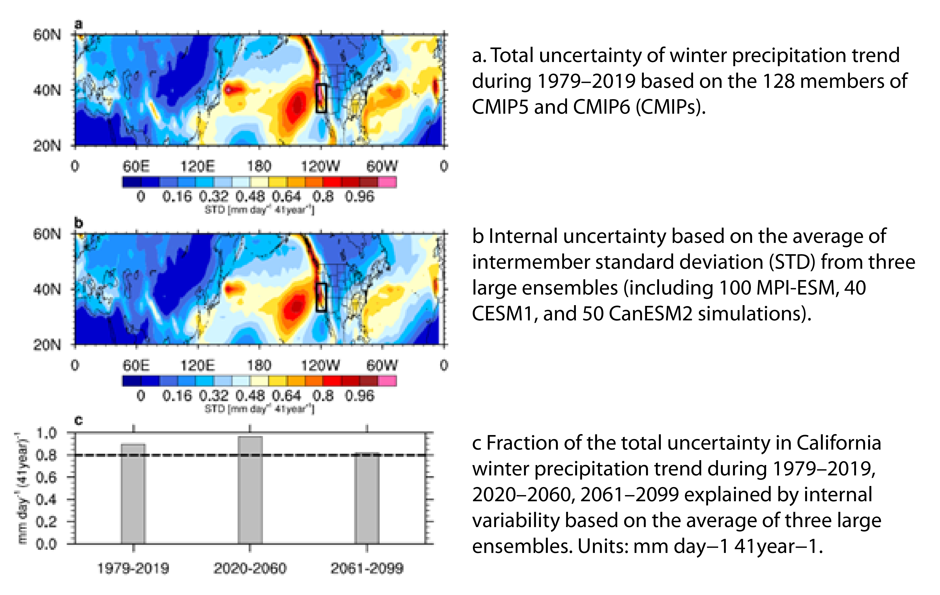
Fig. 1 Effect of internal variability on the large uncertainty of winter precipitation decadal trends over California. (link) 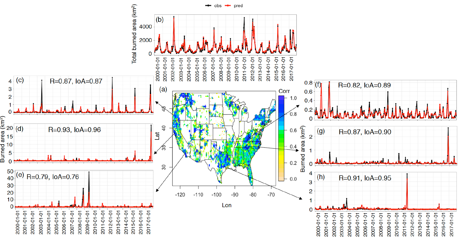
Figure 2. (a) The map of temporal correlation between observed and predicted burned area for each grid. Time series of observed (black) and predicted (red) burned area (b) average across the CONUS, and at grids of (c) lon: 121.625°W, lat: 44.375°, (d) lon: 122.375°W, lat: 38.375°N, (e) lon: 118.375°W, lat: 34.375°, (f) lon: 82.375°W, lat: 37.125°, (g) lon: 83.625°W, lat: 35.625°N, (h) lon: 97.375°W, lat: 30.375°N. CONUS, contiguous United States. (link) 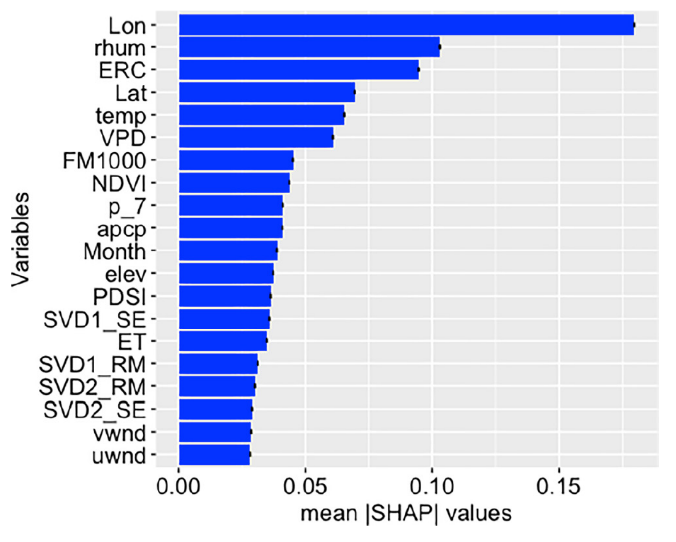
Figure 3. Top 20 variables for the model based on the mean absolute SHAP value with the 95% confidence intervals. SHAP, Shapley additive explanation. (link)