Global Water and Nitrogen Scarcity and Role of Trade

Listen here on Spotify | Listen here on Apple Podcast

Episode released on May 30, 2024 
Episode recorded on March 5, 2024

Junguo Liu is the President of North China University of Water Resources and Electric Power in Zhengzhou, Henan Province, China.

Highlights  |  Transcript

1. Review of water scarcity indices includes (Liu et al., EF, 2017): 
   1. Falkenmark Index: water scarcity: ≤1,700 m3 water/capita/yr
      1. High water scarcity: ≤1,000 m3 water/capita/yr
      2. Absolute water scarcity: ≤500 m3 water/capita/yr
   2. Criticality Ratio: water use to availability ratio:
      1. High water stress: water use >40% of available renewable water resources
   3. IWMI Indicator: considers physical and economic water scarcity
   4. Water Footprint: focuses on water consumption rather than withdrawal used in above indices.
2. Water demand for humans and ecosystems (80% of water assigned to ecosystems)
   1. About 4 billion people subjected to water scarcity at least 1 month/yr (50 km grid scale) relative to ~ 2.5 billion people in most previous studies (annual data) (Mekonnen and Hoekstra, Sci Adv., 2016)
3. Increasing spatial and temporal resolution of water scarcity analyses increases number of people subjected to water scarcity.
4. Environmental flow requirements (ecosystem services) of 80% is too high, leading to overestimation of water scarcity. For example environmental flows are estimated to be ~ 25% for rivers in Tanzania (Liu et al., ERL, 2021).
5. Water quality induced water scarcity: concept first introduced by Junguo Liu’s team (Zeng, Liu and Savenije, 2013; Liu et al., Ecol. Ind., 2016), ratio of grey water footprint (volume of water required to dilute contaminants) to freshwater availability. 
6. Quantity, Quality, Environmental flow requirements (QQE) Huangqihai Basin (Mongolia, N China) suffers from water water scarcity from both quantity and quality perspectives: quantity induced scarcity = 1.3 relative to a threshold of 1.0, quality induced scarcity: 14.2 relative to threshold of 1.0, env. flow requirements ~ 26% of natural water flows (Liu et al., Ecol. Ind., 2016).
7. China: quantity induced scarcity prevalent in semiarid N region, quality scarcity in N region and SE region, no scarcity in SW China (Liu et al., ERL, 2021).
8. Tradeoff between economic development in China, reducing poverty (75% of global poverty reduction) and pollution. 
9. China: National Water Pollution Prevention and Control Action Plan, 2015: State Council implemented this, particularly to eliminate black water in urban areas. 
10. Revised Water Pollution Prevention and Control Law effective Jan., 2018. Recent watershed protection laws. 
    1. Yangtze River Protection Law (Mar, 2021)
    2. Yellow River Protection Law (Apr., 2023)
    3. Address pollution at source, recycling water in industry etc and water treatment at discharge points.
11. Sponge city concept, permeable pavement reduces urban stormwater management, 30 cities (Liu et al., Fron. Env. Sci., 2022) selected to highlight program in 2015/2016. Now national scale. Nature based solution including green infrastructure (Palmer et al., Science, 2015).
    1. Goal: 80% of urban areas absorb and reuse ≥70% of rainwater.
    2. Infiltration, detention, retention, purification, and utilization 
    3. Hybrid green/gray solutions: constructed wetlands, wastewater treatment.
12. Shenzhen City, China: 2016: 310 rivers, 159 black and odorous rivers. 2019: eliminate black and odorous rivers
13. Cleaning Maozhou River (Mother river of Shenzhen), restorative targets, monitoring, cleaned up (e.g. NH3 level reduced from 34 mg/L (2015) to 1.3 mg/L (2020) with a stepwise ecological restoration framework (Liu et al., Sci. Bul., 2021; Liu et al., Geo. Sust. 2014)
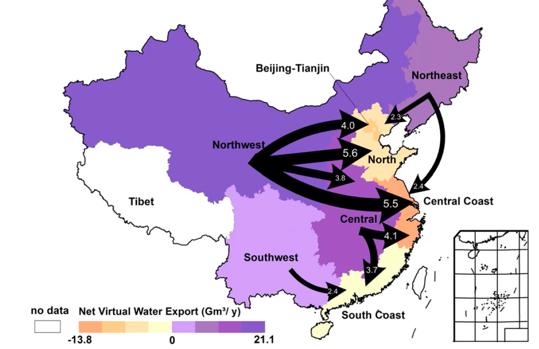
14. Solutions to resolving water scarcity: transport water physically or virtually through food (Zhao et al., PNAS, 2015). 
    1. Physical Transfers of Water in China: 
       1. Year 2007: Virtual water transfers almost 10× > physical water transfers. 
       2. 20 major water transfer projects, 26 km3 (4.5% of natural water supply), 201 km3 virtual water transfers in food (35% of water supply). 
       3. S to N Water Transfer: targeted 45 km3 of water transfers through three routes.
    2. Virtual water transfers in China from semiarid W China to more humid, urbanized E China, alleviating water scarcity for many eastern part of China but amplifying water scarcity in importing regions (Fig. 1). 
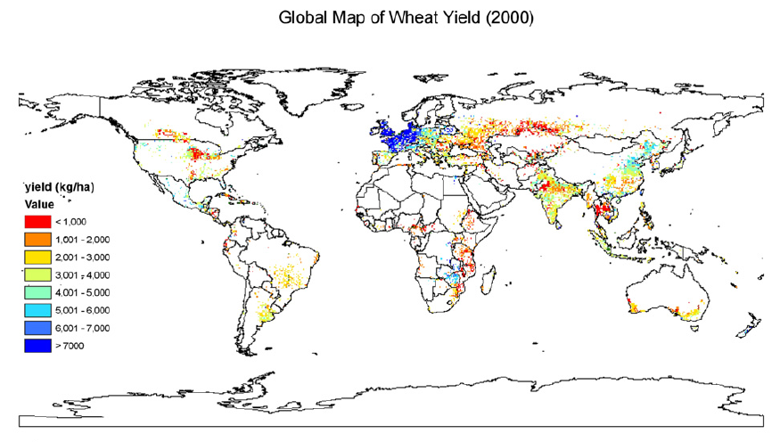
15. Global food trade: wheat production, analyzed using GEPIC (GIS based Env. Policy Integ. Climate) code (Fig. 2) (Liu et al., Ag. Syst., 2007).
16. Crop water productivity: crop tonnage/unit of water consumed, high wheat yields in W and E EU and N China, lowest yields Sub-Saharan Africa (SSA).
17. Modeled potential yield with optimal water and fertilizer application: 
    1. EU potential yield (7,000 kg/ha) and crop water prod. 1.2 kg/m3.
    2. African countries potential yield (5,000-9,000 kg/ha) and crop water prod. 1.2-1.8 kg/m3.
18. African countries may significantly raise crop yields as well as crop water prod by increasing water and fertilizer application.
19. International wheat trade saves water: Data year 2000, global virtual water export 160 km3 (USA, Canada, France, AU, and Argentina), water required to grow those crops in importing countries (Brazil, Italy, Iran, Japan, and Algeria), 240 km3.
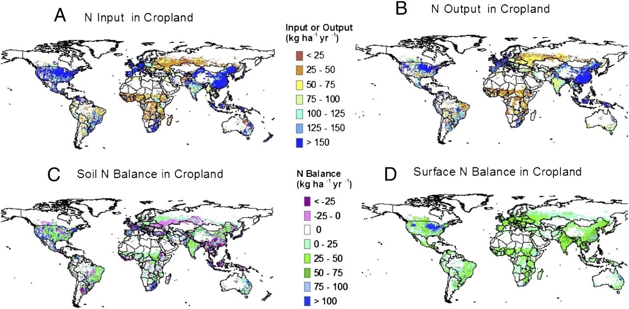
20. Global N Cycle (Liu et al., PNAS, 2010): 10 km grid, N input to crops: 536 trillion g (Tg), dominated by mineral N fertilizer (~50%) (Fig. 3)
21. Cropland output: 150 Tg of N, 35% in harvested crops, 20% crop residue, 16% lost leaching, 15% soil erosion, 14% gaseous emissions. 
22. African countries, 80% N scarcity. N scarcity: ≤9 kg/capita/yr; N stress: 9 – 15 kg/capita/yr.
23. Globally N recovery rate: 60%, 40% lost, ecosystem health impacts. 
24. Fertilizers are expensive in Africa, rely in imports, transport infrastructure poor and expensive.