Listen here on Spotify | Listen here on Apple Podcast
Episode released on July 24, 2025
Episode recorded on April 25, 2025
Image

Yadu Pokhrel describes the application of global hydrologic modeling with machine learning to understand water resources dynamics.
Yadu Pokhrel is a Professor at the Department of Civil and Environmental Engineering at Michigan State University. His research uses global hydrologic models and machine learning to assess water resources within the context of droughts and floods and human intervention.
Highlights | Transcript
Colorado River Basin and application of global models (CLM-2).
- Colorado River Basin, subjected to multidecadal drought with lakes Powell and Mead currently at ~ 30% of capacity (Fig. 1) (Scanlon et al., 2025).
- Pokhrel working on NSF project applying the Community Land Model (CLM, ver. 5) to simulate water resources in the Colorado River Basin.
- Project involves multiple stakeholders: US Bureau of Reclamation, California Dept. Water Resources etc.
- The Community Land Model (CLM) is the land component of the parent climate model, Community Earth System Model (CESM ver. 2) that includes land, atmosphere, and ocean (Fig. 2).
- CLM simulates biophysical and biogeochemical processes along with human interventions.
- In the Colorado River Basin Project, the CLM model was used with river flood and reservoir routing model called CaMa flood (Catchment-based Macro-scale Floodplain) model. The model also simulates irrigation water demand.
- CLM is housed, maintained and released by the National Center for Atmospheric Research (NCAR). NCAR is under UCAR (University Center for Atmospheric Research) and collaborates with universities globally.
- One component of the Colorado River Basin project is to simulate the naturalized flows (no human intervention, no diversions or return flows) at Lees Ferry (Fig. 3), which is the junction between the Upper and Lower Colorado River basins.
- CLM version applied to Colorado uses a 5 km grid, versus 50 km grid for original CLM.
- Simulation of flow at Lees Ferry was originally poor. CLM is a process-based model with 230+ parameters; therefore, it is difficult to determine what parameters to modify to improve model fit.
- Applied artificial intelligence (AI) and machine learning (ML) to determine which parameters control flow in the basin. Reduced 230 parameters to ~30 important parameters. Further reduced to 7 parameters that are most important for modeling surface runoff.
- Then they used emulators to reproduce naturalized flow in Lees Ferry.
- Model parameter optimization often focused on annual simulations; however, simulating seasonal flows and snowmelt is much more challenging.
- Traditionally we have used process-based models to simulate hydrology. More recently there has been a shift to data driven models. However, there are advantages and disadvantages to each approach. The hybrid approach that Pokhrel describes includes the advantages of both approaches by providing process-based explanations while reducing computational intensity.
- A total of 85% of runoff at Lee’s Ferry comes from 15% of the area in the Upper Colorado River Basin.
- Reservoir operations are critical for accurate simulation of the Colorado Basin. Hanasaki incorporated reservoir operations into his global hydrologic model in 2006 (Hanasaki et al., 2006). Pokhrel incorporated that approach to reservoir operations into MATSIRO (Japanese climate model).
- Reservoir operations classified as follows for modeling:
- Hydropower, water continuously released, as shown by flat hydrograph downstream of Lake Mead.
- Irrigation, water release based on downstream irrigation demand.
- Other, flood control, navigation, recreation.
- To simulate reservoirs in the Colorado River Basin, Pokhrel and colleagues first applied generic scheme from Hanasaki and then improved it with data on reservoir operations in the US from Turner et al. (2021).
Global Model Intercomparison Projects
- We rely heavily on output of global models. Assessing their reliability through model comparisons is important.
- Inter-Sectoral Impact Model Intercomparison Project (ISIMIP) initiated in 2012, 18 sectors now (e.g., hydrology, lakes, fire, biodiversity etc).
- Pokhrel and Gosling: coordinators of ISIMIP.
- 2013 – 2014: MIP Fast Track using observation-based datasets with initial focus on runoff and streamflow (Schewe et al. 2014).
- Looking at future predictions with climate change: evaluate variability among models, 8 different models with three Global Climate Models (GCMs) plus different realizations: 85 realizations.
- 66% of realizations indicate that global Terrestrial Water Storage will decline in the 21st century, leading to extreme to exceptional droughts (Pokhrel et al. 2021).
Climate Model Intercomparison Projects (CMIP)
- CMIP models also include hydrologic models, some are included in ISIMIP. Climate models generally coarse resolution, ~200 km. These models focus on climate.
- Three types of models:
- Land Surface Models, land component of climate models (e.g., CLM, MATSIRO)
- Global Hydrological Models, developed independent of climate models (e.g., PCR-GLOBWB, WaterGAP)
- Vegetation Dynamic Models (LJP-ML, Lund Potsdam Jena Managed Land)
- ISIMIP models generally finer resolution than climate models (~ 0.5 degree, ~ 50 km at the Equator)
- Initially ISIMIP focused on fluxes, runoff, streamflow, ET, then added storage, Terrestrial Water Storage to compare with GRACE satellite data.
- Gradually incorporating human intervention into models. WaterGAP comprehensive human water use for many sectors, MATSIRO incorporating reservoirs and irrigation
- Irrigation: 70% global water withdrawal, 90% water consumption
- Simulating irrigation: Simulate Potential ET and Actual ET, if AET < PET, increase AET to closely match PET, the gap is irrigation. Only GHMs simulate PET.
- LSMs do not simulate PET but simulate the energy balance. Use Soil Moisture Deficit to estimate irrigation in LSMs. Increasing soil moisture to field capacity to simulate irrigation.
- Use satellite data, such as Soil Moisture Active Passive (SMAP) satellites to constrain irrigation simulation (McDermid et al., 2023)
- Irrigation Model Intercomparison Project: IRRMIP,
- Initial simulations used prescribed crops. 13 – 14 vegetation types, one is crop.
- CLM now includes a crop model that simulates crop phenology (planting, growing, harvesting)
- ABIM: Agent Based Irrigation Model, agronomy-based crop model considers stresses from heat, water and nutrients.
- Can simulate crop yield and link to food security.
- Simulating human intervention, initially focused on water demand within a cell, first tap into available surface water, then groundwater.
- In US, use water sources for sectoral water uses, surface water, and groundwater.
- Developed various indices, such as water scarcity index.
- Some models consider renewable vs nonrenewable water.
- Many consider water to be unlimited.
- Others consider economic factors in terms of depth to water and costs of well drilling and extraction.
Millions of abandoned wells in India, infeasible to pump even with subsidized electricity.
Image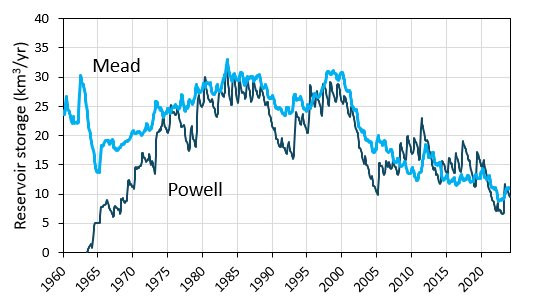
Figure 1. Time series of reservoir storage in Lake Powell and Lake Mead showing large declines related to recent droughts since 2000. Image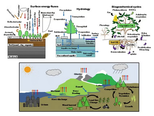
Figure 2. Community Land Model which is the land model for the Community Earth System Model (CESM). link Image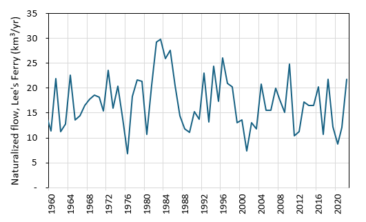
Figure 3. Naturalized flow at Lee’s Ferry, junction between Upper and Lower Colorado River Basins (Scanlon et al., 2025).